SequentialSystem#

class optika.systems.SequentialSystem(surfaces, object=None, sensor=None, axis_surface='surface', grid_input=None, transformation=None, kwargs_plot=None)[source]#

Bases: AbstractSequentialSystem

A sequential optical system is a composition of a sequence of optika.surfaces.AbstractSurface instances and a default grid to sample them with.

Examples

Here is an example of a simple Newtonian telescope, with a parabolic primary mirror, a 45 degree fold mirror, and a detector.

import dataclasses
import matplotlib.pyplot as plt
import astropy.units as u
import astropy.visualization
import named_arrays as na
import optika

# store the coordinates of the primary mirror, fold mirror,
# and sensor, so we can determine the focal length of the
# primary mirror.
primary_mirror_z = 200 * u.mm
fold_mirror_z = 50 * u.mm
sensor_x = 50 * u.mm

# Define the front aperture surface.
front = optika.surfaces.Surface(
    name="front",
)

# Define the parabolic primary mirror.
primary_mirror = optika.surfaces.Surface(
    name="mirror",
    sag=optika.sags.ParabolicSag(
        focal_length=-(primary_mirror_z - fold_mirror_z + sensor_x),
    ),
    aperture=optika.apertures.RectangularAperture(40 * u.mm),
    material=optika.materials.Mirror(),
    is_pupil_stop=True,
    transformation=na.transformations.Cartesian3dTranslation(
        z=primary_mirror_z,
    ),
)

# Define the flat fold mirror which directs light
# to the detector surface.
fold_mirror = optika.surfaces.Surface(
    name="fold_mirror",
    aperture=optika.apertures.RectangularAperture(25 * u.mm),
    material=optika.materials.Mirror(),
    transformation=na.transformations.TransformationList([
        na.transformations.Cartesian3dRotationY((90 + 45) * u.deg),
        na.transformations.Cartesian3dTranslation(
            z=fold_mirror_z,
        ),
    ]),
)

# Define the central obscuration, the back face
# of the fold mirror which blocks some of the
# incoming light.
obscuration = optika.surfaces.Surface(
    name="obscuration",
    aperture=dataclasses.replace(fold_mirror.aperture, inverted=True),
    transformation=fold_mirror.transformation,
)

# define the imaging sensor surface
sensor = optika.sensors.ImagingSensor(
    name="sensor",
    width_pixel=20 * u.um,
    axis_pixel=na.Cartesian2dVectorArray("detector_x", "detector_y"),
    num_pixel=na.Cartesian2dVectorArray(128, 128),
    timedelta_exposure=1 * u.s,
    transformation=na.transformations.TransformationList([
        na.transformations.Cartesian3dRotationY(-90 * u.deg),
        na.transformations.Cartesian3dTranslation(
            x=-sensor_x,
            z=fold_mirror_z,
        ),
    ]),
    is_field_stop=True,
)

# Define the grid of normalized field coordinates,
field = na.Cartesian2dVectorLinearSpace(
    start=-1,
    stop=1,
    axis=na.Cartesian2dVectorArray("field_x", "field_y"),
    num=5,
    centers=True,
)

# Define the grid of normalized pupil coordinates
# in a similar fashion to the normalized field
# coordinates
pupil = na.Cartesian2dVectorLinearSpace(
    start=-1,
    stop=1,
    axis=na.Cartesian2dVectorArray("pupil_x", "pupil_y"),
    num=5,
    centers=True,
)

# define the optical system using the surfaces
# and the normalized field/pupil coordinates
system = optika.systems.SequentialSystem(
    surfaces=[
        front,
        obscuration,
        primary_mirror,
        fold_mirror,
    ],
    sensor=sensor,
    grid_input=optika.vectors.ObjectVectorArray(
        wavelength=500 * u.nm,
        field=field,
        pupil=pupil,
    ),
)

# plot the system
with astropy.visualization.quantity_support():
    fig, ax = plt.subplots(constrained_layout=True)
    ax.set_aspect("equal")
    system.plot(
        ax=ax,
        components=("z", "x"),
        kwargs_rays=dict(
            color="tab:blue",
        ),
        color="black",
        zorder=10,
    )

../_images/optika.systems.SequentialSystem_0_0.png

Using this model, we can simulate an image of an airforce target

# Define the number of points to sample
num_field = 2 * system.sensor.num_pixel

# Define the scene as an airforce target.
# Note how the coordinates (inputs) are defined on
# cell vertices and the values (outputs) are
# defined on cell centers.
scene = na.FunctionArray(
    inputs=na.SpectralPositionalVectorArray(
        wavelength=na.linspace(530, 531, axis="wavelength", num=2) * u.nm,
        position=na.Cartesian2dVectorLinearSpace(
            start=system.field_min,
            stop=system.field_max,
            axis=na.Cartesian2dVectorArray("field_x", "field_y"),
            num=num_field + 1,
        ),
    ),
    outputs=optika.targets.airforce(
        axis_x="field_x",
        axis_y="field_y",
        num_x=num_field.x,
        num_y=num_field.y,
    ) * 100 * u.photon / u.s / u.m ** 2 / u.arcsec ** 2 / u.nm,
)

# Simulate an image of the scene using the optical system
image = system.image(scene)

# Plot the original scene and the simulated image
with astropy.visualization.quantity_support():
    fig, ax = plt.subplots(
        ncols=2,
        figsize=(8, 5),
        constrained_layout=True,
    )
    mappable_scene = na.plt.pcolormesh(
        scene.inputs.position,
        C=scene.outputs.value,
        ax=ax[0],
    )
    mappable_image = na.plt.pcolormesh(
        image.inputs.position,
        C=image.outputs.value.sum("wavelength"),
        ax=ax[1],
    )
    cbar_0 = fig.colorbar(
        mappable=mappable_scene.ndarray.item(),
        ax=ax[0],
        location="top",
    )
    cbar_0.set_label(f"radiance ({scene.outputs.unit:latex_inline})")
    cbar_1 = fig.colorbar(
        mappable=mappable_image.ndarray.item(),
        ax=ax[1],
        location="top",
    )
    cbar_1.set_label(f"measured charge ({image.outputs.unit:latex_inline})")
    ax[0].set_aspect("equal")
    ax[1].set_aspect("equal")

../_images/optika.systems.SequentialSystem_1_0.png

The result is flipped vertically and horizontally due to the layout of the optical system. The noise on the image is from the stratified random sampling used to generate the grid of rays traced through the system, there is no additional noise sources, such as photon shot noise in this simulation.

Attributes

`axis_surface`	The name of the logical axis representing the sequence of surfaces.
`field_max`	The upper right corner of this optical system's field of view.
`field_min`	The lower left corner of this optical system's field of view.
`field_stop`	The field stop surface.
`grid_input`	The input grid to sample with rays.
`index_field_stop`	The index of the field stop in `surfaces_all`.
`index_pupil_stop`	The index of the pupil stop in `surfaces_all`.
`kwargs_plot`	Additional keyword arguments used by default in `plot()`.
`object`	The external object being imaged or illuminated by this system.
`object_is_at_infinity`	A boolean flag indicating if the object is at infinity.
`pupil_max`	The upper right corner of this optical system's entrance pupil in physical units.
`pupil_min`	The lower left corner of this optical system's entrance pupil in physical units.
`pupil_stop`	The pupil stop surface.
`rayfunction_default`	Computes the rays in local coordinates at the last surface in the system as a function of input wavelength and position using `grid_input`.
`rayfunction_stops`	A rayfunction defined on the input surface of the optical system, which is designed to exactly strike the borders of both the field stop and the pupil stop.
`sensor`	The imaging sensor that measures the light captured by this system.
`shape`	The array shape of this object.
`surfaces`	A sequence of surfaces representing this optical system.
`surfaces_all`	Concatenate `object` with `surfaces` into a single list of surfaces.
`transformation`	A optional coordinate transformation to apply to the entire optical system.

Methods

`__init__`(surfaces[, object, sensor, ...])
`image`(scene[, pupil, axis_wavelength, ...])	Forward model of the optical system.
`plot`([ax, transformation, components, ...])	Plot the surfaces of the system and the default raytrace.
`rayfunction`([intensity, wavelength, field, ...])	Given the wavelength, field position, and pupil position of some input rays, trace those rays through the system and return the resulting rays in local coordinates of the sensor (if it exists).
`raytrace`([intensity, wavelength, field, ...])	Given the wavelength, field position, and pupil position of some input rays, trace those rays through the system and return the result in global coordinates, optionally including all intermediate rays.
`spot_diagram`([figsize, s, cmap])	Create a spot diagram of the rays at each field point to inspect the performance of this optical system.
`to_dxf`(file, unit[, transformation])
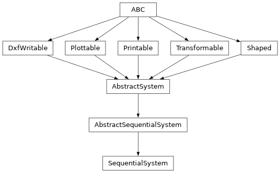
`to_string`([prefix])	Public-facing version of the `__repr__` method that allows for defining a prefix string, which can be used to calculate how much whitespace to add to the beginning of each line of the result.

Inheritance Diagram

Parameters:

surfaces (Sequence[AbstractSurface])
object (AbstractSurface)
sensor (AbstractImagingSensor)
axis_surface (str)
grid_input (ObjectVectorArray)
transformation (None | AbstractTransformation)
kwargs_plot (None | dict[str, Any])

image(scene, pupil=None, axis_wavelength=None, axis_field=None, axis_pupil=None, integrate=True, noise=True)#

Forward model of the optical system. Maps the given spectral radiance of a scene to detector counts.

Parameters:

scene (FunctionArray[SpectralPositionalVectorArray, AbstractScalar]) – The spectral radiance of the scene as a function of wavelength and field position. The inputs must be cell vertices.
pupil (None | AbstractCartesian2dVectorArray) – The vertices of the pupil grid in either normalized or physical coordinates. If None (the default), the pupil grid will only have one cell.
axis_wavelength (None | str) – The logical axis of scene corresponding to changing wavelength coordinate. If None, set(scene.inputs.wavelength.shape) - set(self.shape), should have only one element.
axis_field (None | tuple[str, str]) – The two logical axes of scene corresponding to changing field coordinate. If None, set(scene.inputs.position.shape) - set(self.shape) - {axis_wavelength}, should have exactly two elements.
axis_pupil (None | tuple[str, str]) – The two logical axes of pupil corresponding to changing pupil coordinate. If None, set(pupil.shape) - set(self.shape) - {axis_wavelength,} - set(axis_field), should have exactly two elements. If pupil is None, this parameter is ignored.
integrate (bool) – Whether to integrate the wavelength axis. Real images usually have the wavelength axis integrated since they use a black/white sensor, but it can be useful to leave the wavelengths separate for introspective purposes.
noise (bool) – Whether to add noise to the result.

Return type:

FunctionArray[SpectralPositionalVectorArray, AbstractScalar]

plot(ax=None, transformation=None, components=None, plot_rays=True, plot_rays_vignetted=False, kwargs_rays=None, **kwargs)#

Plot the surfaces of the system and the default raytrace.

Parameters:

ax (None | Axes | ScalarArray[ndarray[tuple[Any, ...], dtype[_ScalarT]]]) – The matplotlib axes on which to plot the system
transformation (None | AbstractTransformation) – Any additional transformation to apply to the system before plotting.
components (None | tuple[str, ...]) – The vector components to plot if ax is 2-dimensional.
plot_rays (bool) – Boolean flag indicating whether to plot the rays.
plot_rays_vignetted (bool) – Boolean flag indicating whether to plot the vignetted rays.
kwargs_rays (None | dict[str, Any]) – Any additional keyword arguments to use when plotting the rays.
kwargs – Any additional keyword arguments to use when plotting the surfaces.

Return type:

AbstractScalar | dict[str, AbstractScalar]

rayfunction(intensity=None, wavelength=None, field=None, pupil=None, normalized_field=True, normalized_pupil=True)#

Given the wavelength, field position, and pupil position of some input rays, trace those rays through the system and return the resulting rays in local coordinates of the sensor (if it exists).

Parameters:

intensity (None | float | Quantity | AbstractScalar) – The energy density of the input rays.
wavelength (None | Quantity | AbstractScalar) – The wavelengths of the input rays. If None (the default), self.grid_input.wavelength will be used.
field (None | AbstractCartesian2dVectorArray) – The field positions of the input rays, in either normalized or physical units. If None (the default), self.grid_input.field will be used.
pupil (None | AbstractCartesian2dVectorArray) – The pupil positions of the input rays, in either normalized or physical units. If None (the default), self.grid_input.pupil will be used.
normalized_field (bool) – A boolean flag indicating whether the field parameter is given in normalized or physical units.
normalized_pupil (bool) – A boolean flag indicating whether the pupil parameter is given in normalized or physical units.

Return type:

RayFunctionArray