Prime Focus Telescope Tutorial

The prime focus telescope is one of the simplest telescope designs since it has only one reflection and no obscuration surfaces (ignoring the small obscuration from the sensor). It works by placing a sensor at the focus of a parabolic primary mirror. This tutorial will demonstrate how to model a prime focus telescope using optika and investigate its performance

import matplotlib.pyplot as plt
import astropy.units as u
import astropy.visualization
import named_arrays as na
import optika

Primary mirror

We’ll start by defining the primary mirror aperture radius

radius_aperture = 100 * u.mm

and the \(f\)-number of the primary mirror

f_number = 5

So the focal length of the primary is then

focal_length = f_number * radius_aperture
focal_length

$500 \; \mathrm{mm}$

We can specify a parabolic sag profile for our primary mirror using the optika.sags.ParabolicSag class

sag_primary = optika.sags.ParabolicSag(-focal_length)

For simplicity, we will consider the primary mirror to be a perfectly-reflective mirror, which we can reprsent with optika.materials.Mirror.

material_primary = optika.materials.Mirror()

To specify a circular apeture for our primary mirror, we can use optika.apertures.CircularAperture.

aperture_primary = optika.apertures.CircularAperture(radius_aperture)

Finally, we can specify the position and orientation of the primary mirror using the named_arrays.transformations module. To translate the primary mirror one focal length away from the origin, we use named_arrays.transformations.Cartesian3dTranslation.

translation_primary = na.transformations.Cartesian3dTranslation(z=focal_length)

We can combine the sag profile, aperture shape, material type, and coordinate transformation into one object to represent the primary mirror, an instance of optika.surfaces.Surface.

primary = optika.surfaces.Surface(
    name="primary",
    sag=sag_primary,
    material=material_primary,
    aperture=aperture_primary,
    transformation=translation_primary,
    is_pupil_stop=True,
)

The is_pupil_stop=True statement in the previous cell sets the primary mirror as the pupil stop, the surface that controls the size of the entrance pupil.

Sensor

If the size of each pixel in the sensor is

width_pixel = 15 * u.um

The number of pixels along each axis is

num_pixel = na.Cartesian2dVectorArray(256, 256)

The name of each axis of the pixel array is

axis_pixel = na.Cartesian2dVectorArray("detector_x", "detector_y")

In optika, the surface normal should be antiparallel to the incident light. To accomplish this the sensor needs to be rotated 180 degrees.

rotation_sensor = na.transformations.Cartesian3dRotationY(180 * u.deg)

Putting it all together, we can represent the sensor using optika.sensors.ImagingSensor

sensor = optika.sensors.ImagingSensor(
    name="sensor",
    width_pixel=width_pixel,
    axis_pixel=axis_pixel,
    num_pixel=num_pixel,
    transformation=rotation_sensor,
    is_field_stop=True,
)

The is_field_stop=True statement in the previous cell sets the sensor as the field stop, the surface that controls the size of the field of view

Input rays

The position and direction of the input rays is specified in terms of normalized coordinates. We can specify a uniform normlized pupil grid withSS

pupil = na.Cartesian2dVectorLinearSpace(
    start=-1,
    stop=1,
    axis=na.Cartesian2dVectorArray("px", "py"),
    num=5,
    centers=True,
)

a normalized field grid with

field = na.Cartesian2dVectorLinearSpace(
    start=-1,
    stop=1,
    axis=na.Cartesian2dVectorArray("fx", "fy"),
    num=5,
    centers=True,
)

and assume a constant wavelength

wavelength = 500 * u.nm

optika provides a vector type for representing a point in wavelength/field/pupil space, optika.vectors.ObjectVectorArray

grid_input = optika.vectors.ObjectVectorArray(
    wavelength=wavelength,
    field=field,
    pupil=pupil,
)

Building the system

optika.systems.SequentialSystem is a composition of the optical surfaces and the input ray grid.

system = optika.systems.SequentialSystem(
    surfaces=[
        primary,
    ],
    sensor=sensor,
    grid_input=grid_input,
)

We can plot the system using the optika.systems.SequentialSystem.plot() method.

# plot the system
with astropy.visualization.quantity_support():
    fig, ax = plt.subplots(constrained_layout=True)
    ax.set_aspect("equal")
    system.plot(
        ax=ax,
        components=("z", "y"),
        kwargs_rays=dict(
            color="tab:blue",
        ),
        color="black",
        zorder=10,
    )

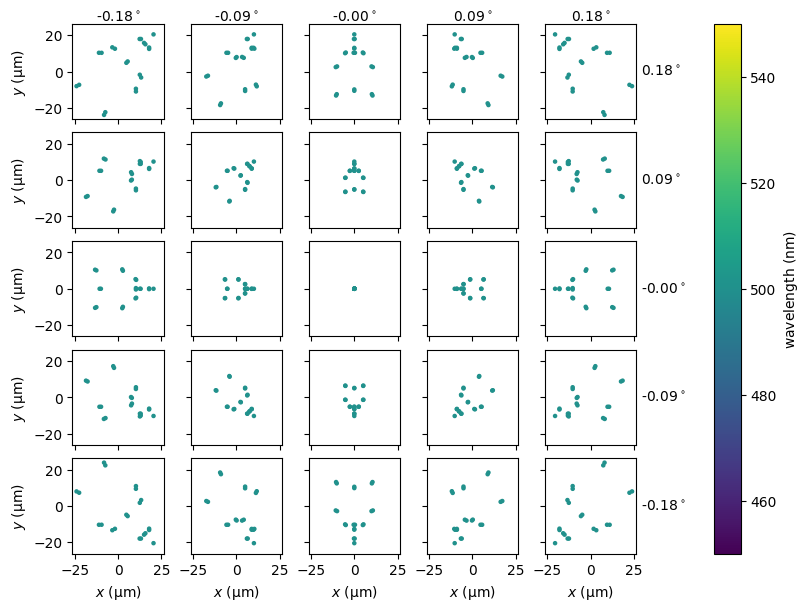
Spot Diagrams

We can plot a spot diagram for each field angle using the spot_diagram() method of SequentialSystem.

fig, ax = system.spot_diagram()