SinusoidalRulings#

class optika.rulings.SinusoidalRulings(spacing, depth, diffraction_order)[source]#

Bases: AbstractRulings

A ruling profile described by a sinusoidal wave.

Examples

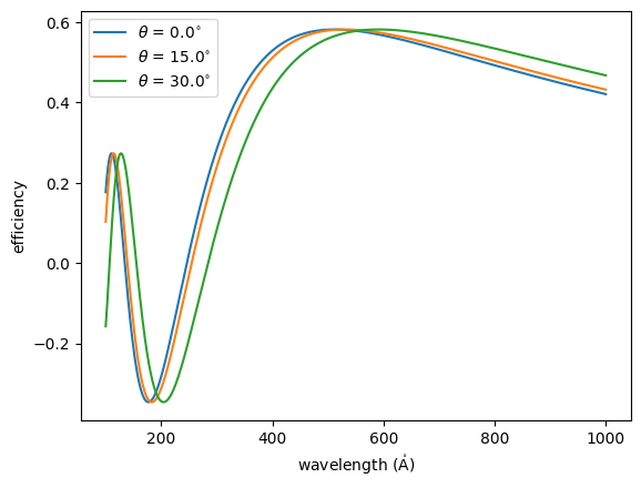
Compute the 1st-order groove efficiency of sinusoidal rulings with a groove density of 2500 grooves/mm and a groove depth of 15 nm.

import numpy as np
import matplotlib.pyplot as plt
import astropy.units as u
import named_arrays as na
import optika

# Define the groove density
density = 2500 / u.mm

# Define the groove depth
depth = 15 * u.nm

# Define ruling model
rulings = optika.rulings.SinusoidalRulings(
    spacing=1 / density,
    depth=depth,
    diffraction_order=1,
)

# Define the wavelengths at which to sample the groove efficiency
wavelength = na.geomspace(100, 1000, axis="wavelength", num=1001) * u.AA

# Define the incidence angles at which to sample the groove efficiency
angle = na.linspace(0, 30, num=3, axis="angle") * u.deg

# Define the light rays incident on the grooves
rays = optika.rays.RayVectorArray(
    wavelength=wavelength,
    direction=na.Cartesian3dVectorArray(
        x=np.sin(angle),
        y=0,
        z=np.cos(angle),
    ),
)

# Compute the efficiency of the grooves for the given wavelength
efficiency = rulings.efficiency(
    rays=rays,
    normal=na.Cartesian3dVectorArray(0, 0, -1),
)

# Plot the groove efficiency as a function of wavelength
fig, ax = plt.subplots()
angle_str = angle.value.astype(str).astype(object)
na.plt.plot(
    wavelength,
    efficiency,
    ax=ax,
    axis="wavelength",
    label=r"$\theta$ = " + angle_str + f"{angle.unit:latex_inline}",
);
ax.set_xlabel(f"wavelength ({wavelength.unit:latex_inline})");
ax.set_ylabel(f"efficiency");
ax.legend();

../_images/optika.rulings.SinusoidalRulings_0_0.png

Attributes

`depth`	Depth of the ruling pattern.
`diffraction_order`	The diffraction order to simulate.
`shape`	The array shape of this object.
`spacing`	Spacing between adjacent rulings at the given position.
`spacing_`	A normalized version of `spacing` that is guaranteed to be an instance of `optika.rulings.AbstractRulingSpacing`.

Methods

`__init__`(spacing, depth, diffraction_order)
`efficiency`(rays, normal)	The fraction of light diffracted into a given order.
`incident_effective`(rays, normal)	Compute the effective propagation direction of the given rays using `incident_effective()`.
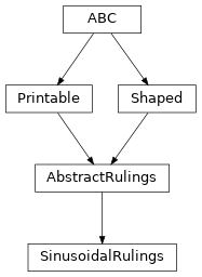
`to_string`([prefix])	Public-facing version of the `__repr__` method that allows for defining a prefix string, which can be used to calculate how much whitespace to add to the beginning of each line of the result.

Inheritance Diagram

Parameters:

spacing (Quantity | AbstractScalar | AbstractRulingSpacing)
depth (Quantity | AbstractScalar)
diffraction_order (int | AbstractScalar)

efficiency(rays, normal)[source]#

The fraction of light diffracted into a given order.

Calculated using the expression given in Table 1 of Magnusson and Gaylord [1978].

Parameters:

rays (RayVectorArray) – The light rays incident on the rulings
normal (AbstractCartesian3dVectorArray) – The vector normal to the surface on which the rulings are placed.

Return type:

float | AbstractScalar

Notes

The theoretical efficiency of thin (wavelength much smaller than the groove spacing), sinusoidal rulings is given by Table 1 of Magnusson and Gaylord [1978],

\[\eta_i = J_i^2(2 \gamma)\]

where \(\eta_i\) is the groove efficiency for diffraction order \(i\), \(J_i(x)\) is a Bessel function of the first kind, \(\gamma = \pi d n_1 / \lambda \cos \theta\) is the normalized amplitude of the fundamental grating, \(d\) is the thickness of the grating, \(n_1\) is the amplitude of the fundamental grating, \(\lambda\) is the free-space wavelength of the incident light, and \(\theta\) is the angle of incidence inside the medium.

incident_effective(rays, normal)#

Compute the effective propagation direction of the given rays using incident_effective().

Parameters:

rays (RayVectorArray) – The light rays incident on the rulings
normal (AbstractCartesian3dVectorArray) – The vector normal to the surface on which the rulings are placed.

Return type:

RayVectorArray

to_string(prefix=None)#

Public-facing version of the __repr__ method that allows for defining a prefix string, which can be used to calculate how much whitespace to add to the beginning of each line of the result.

Parameters:: prefix (None | str) – an optional string, the length of which is used to calculate how much whitespace to add to the result.
Return type:: str

depth: Quantity | AbstractScalar = <dataclasses._MISSING_TYPE object>#: Depth of the ruling pattern.

diffraction_order: int | AbstractScalar = <dataclasses._MISSING_TYPE object>#: The diffraction order to simulate.

property shape: dict[str, int]#: The array shape of this object.

spacing: Quantity | AbstractScalar | AbstractRulingSpacing = <dataclasses._MISSING_TYPE object>#: Spacing between adjacent rulings at the given position.

property spacing_: AbstractRulingSpacing#: A normalized version of spacing that is guaranteed to be an instance of optika.rulings.AbstractRulingSpacing.