quantum_efficiency_effective

optika.sensors.quantum_efficiency_effective(wavelength, direction=1, n=1, thickness_oxide=<Quantity 50. Angstrom>, thickness_implant=<Quantity 2317. Angstrom>, thickness_substrate=<Quantity 7. um>, cce_backsurface=0.21, chemical_oxide='SiO2', chemical_substrate='Si', roughness_oxide=<Quantity 0. nm>, roughness_substrate=<Quantity 0. nm>)

Calculate the effective quantum efficiency of a backilluminated detector.

Parameters:

• wavelength (Quantity | AbstractScalar) – The wavelength of the incident light in vacuum.

• direction (float | AbstractScalar) – The cosine of the incidence angle. Default is normal incidence.

• n (complex | AbstractScalar) – The complex index of refraction of the ambient medium.

• thickness_oxide (Quantity | AbstractScalar) – The thickness of the oxide layer on the back surface of the sensor. Default is the value given in Stern et al. [1994].

• thickness_implant (Quantity | AbstractScalar) – The thickness of the implant layer. Default is the value given in Stern et al. [1994].

• thickness_substrate (Quantity | AbstractScalar) – The thickness of the silicon substrate. Default is the value given in Stern et al. [1994].

• cce_backsurface (Quantity | AbstractScalar) – The differential charge collection efficiency on the back surface of the sensor. Default is the value given in Stern et al. [1994].

• chemical_oxide (str | AbstractChemical) – The chemical composition of the oxide layer. The default is to assume the oxide layer is silicon dioxide.

• chemical_substrate (str | AbstractChemical) – Optional complex refractive index of the implant region and substrate. The default is to assume the substrate is made from silicon.

• roughness_oxide (Quantity | AbstractScalar) – The RMS roughness the oxide layer surface.

• roughness_substrate (Quantity | AbstractScalar) – The RMS roughness of the substrate surface.

Return type:

AbstractScalar

Examples

Reproduce Figure 12 from Stern et al. [1994], the modeled quantum efficiency of a Tektronix TK512CB \(512 \times 512\) pixel backilluminated CCD.

import matplotlib.pyplot as plt
import numpy as np
import astropy.units as u
import named_arrays as na
import optika

# Define an array of wavelengths with which to sample the EQE
wavelength = na.geomspace(10, 10000, axis="wavelength", num=1001) * u.AA

# Compute the effective quantum efficiency
eqe = optika.sensors.quantum_efficiency_effective(
    wavelength=wavelength,
)

# Compute the maximum theoretical quantum efficiency
eqe_max = optika.sensors.quantum_efficiency_effective(
    wavelength=wavelength,
    cce_backsurface=1,
)

# Plot the effective and maximum quantum efficiency
fig, ax = plt.subplots(constrained_layout=True)
na.plt.plot(
    wavelength,
    eqe,
    ax=ax,
    label="effective quantum efficiency",
);
na.plt.plot(
    wavelength,
    eqe_max,
    ax=ax,
    label="maximum quantum efficiency",
);
ax.set_xscale("log");
ax.set_xlabel(f"wavelength ({wavelength.unit:latex_inline})");
ax.set_ylabel("efficiency");
ax.legend();

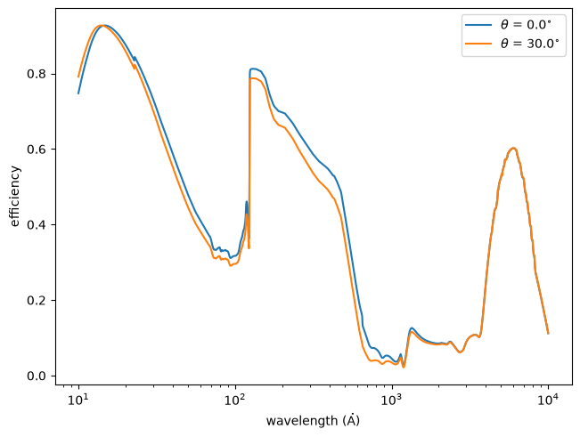
Plot the EQE as a function of wavelength for normal and oblique incidence

import matplotlib.pyplot as plt
import numpy as np
import astropy.units as u
import named_arrays as na
import optika

# Define an array of wavelengths with which to sample the EQE
wavelength = na.geomspace(10, 10000, axis="wavelength", num=1001) * u.AA

# Define the cosines of the incidence angles
angle = na.linspace(0, 30, axis="angle", num=2) * u.deg
direction = np.cos(angle)

eqe = optika.sensors.quantum_efficiency_effective(
    wavelength=wavelength,
    direction=direction,
)

# Plot the results
fig, ax = plt.subplots(constrained_layout=True)
angle_str = angle.value.astype(str).astype(object)
na.plt.plot(
    wavelength,
    eqe,
    ax=ax,
    axis="wavelength",
    label=r"$\theta$ = " + angle_str + f"{angle.unit:latex_inline}",
);
ax.set_xscale("log");
ax.set_xlabel(f"wavelength ({wavelength.unit:latex_inline})");
ax.set_ylabel("efficiency");
ax.legend();

Notes

Stern et al. [1994] defines the effective quantum efficiency as

(1)\[\text{EQE}(\lambda) = A(\lambda) \times \text{CCE}(\lambda),\]

where \(A(\lambda)\) is the absorbtivity of the epitaxial silicon layer for a given wavelength \(\lambda\), and \(\text{CCE}(\lambda)\) is the charge collection efficiency (computed by charge_collection_efficiency()).

References to optika.sensors.quantum_efficiency_effective
quantum_efficiency_effective