e2v_ccd64_thin

optika.sensors.materials.depletion.e2v_ccd64_thin()

A model of the depletion region of a “thin” (20 \(\Omega\)-cm) e2v CCD64 imaging sensor, which uses charge diffusion measurements from Stern et al. [2004] to estimate the thickness of the depletion region.

Examples

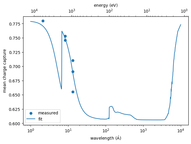
Plot the measured e2v CCD64 measured mean charge capture vs. the fitted mean charge capture.

import matplotlib.pyplot as plt
import astropy.units as u
import astropy.visualization
import named_arrays as na
import optika

# Create a new instance of the e2v CCD64 depletion region model
depletion = optika.sensors.materials.depletion.e2v_ccd64_thin()

# Store the wavelengths at which the MCC was measured
wavelength_measured = depletion.mcc_measured.inputs

# Store the MCC measurements
mcc_measured = depletion.mcc_measured.outputs

# Define a grid of wavelengths with which to evaluate the fitted MCC
wavelength_fit = na.geomspace(1, 10000, axis="wavelength", num=1001) * u.AA
energy_fit = wavelength_fit.to(u.eV, equivalencies=u.spectral())

# Evaluate the fitted MCC using the given wavelengths
mcc_fit = depletion.mean_charge_capture(wavelength_fit)

# Plot the measured QE vs the fitted QE
with astropy.visualization.quantity_support():
    fig, ax = plt.subplots(constrained_layout=True)
    ax2 = ax.twiny()
    ax2.invert_xaxis()
    na.plt.scatter(
        wavelength_measured,
        mcc_measured,
        ax=ax,
        label="measured",
    )
    na.plt.plot(
        wavelength_fit,
        mcc_fit,
        ax=ax,
        label="fit",
    )
    na.plt.plot(
        energy_fit,
        mcc_fit,
        ax=ax2,
        linestyle="None",
    )
    ax.set_xscale("log")
    ax2.set_xscale("log")
    ax.set_xlabel(f"wavelength ({ax.get_xlabel()})")
    ax2.set_xlabel(f"energy ({ax2.get_xlabel()})")
    ax.set_ylabel("mean charge capture")
    ax.legend()

The thickness of the depletion region found by the fit is

depletion.thickness

\[3.5532466 \; \mathrm{\mu m}\]

References to optika.sensors.materials.depletion.e2v_ccd64_thin
e2v_ccd64_thin

Return type:

JanesickDepletionModel