vmr_signal

optika.sensors.vmr_signal(wavelength, absorption=None, thickness_implant=<Quantity 2317. Angstrom>, cce_backsurface=0.21, temperature=<Quantity 300. K>, shot=True, fano=True, pcc=True)

Compute the variance-to-mean ratio (VMR) of the number of electrons measured by the sensor using an analytic expression.

Parameters:

• wavelength (Quantity | ScalarArray) – The vacuum wavelength of the absorbed photons.

• absorption (None | Quantity | AbstractScalar) – The absorption coefficient of the light-sensitive material for the wavelength of interest. If None (the default), the result of optika.chemicals.Chemical.absorption() for silicon will be used.

• thickness_implant (Quantity | AbstractScalar) – The thickness of the implant layer. Default is the value given in Stern et al. [1994].

• cce_backsurface (Quantity | AbstractScalar) – The differential charge collection efficiency on the back surface of the sensor. Default is the value given in Stern et al. [1994].

• temperature (Quantity | ScalarArray) – The temperature of the light-sensitive silicon layer.

• shot (bool) – Whether to include shot noise in the result.

• fano (bool) – Whether to include the Fano noise in the result.

• pcc (bool) – Whether to include noise due to partial charge collection in the result.

Return type:

ScalarArray

Examples

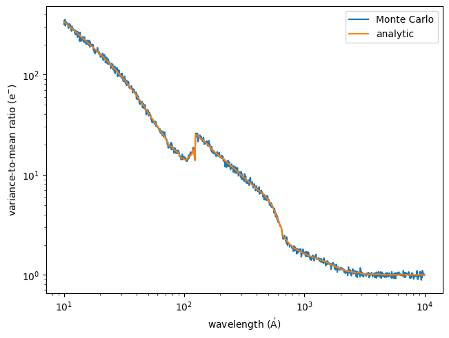
Compute the VMR of the signal analytically and compare to a Monte Carlo approximation

import matplotlib.pyplot as plt
import astropy.units as u
import named_arrays as na
import optika

# Define the number of experiments to perform
num_experiments = 1000

# Define the expected number of photons
# for each experiment
photons_expected = 100 * u.photon

# Define a grid of wavelengths
wavelength = na.geomspace(10, 10000, axis="wavelength", num=1001) * u.AA

# Compute the variance-to-mean ratio of the signal analytically
vmr_signal = optika.sensors.vmr_signal(wavelength)

# Compute the actual number of electrons measured for each experiment
signal = optika.sensors.signal(
    photons_expected=photons_expected,
    wavelength=wavelength,
    shape_random=dict(experiment=num_experiments),
)

# Plot the variance-to-mean ratio of the result
# as a function of wavelength.
fig, ax = plt.subplots(constrained_layout=True)
na.plt.plot(
    wavelength,
    signal.vmr("experiment"),
    ax=ax,
    label="Monte Carlo",
);
na.plt.plot(
    wavelength,
    vmr_signal,
    ax=ax,
    label="analytic"
);
ax.set_xscale("log");
ax.set_yscale("log");
ax.set_xlabel(f"wavelength ({wavelength.unit:latex_inline})");
ax.set_ylabel(f"variance-to-mean ratio ({signal.unit:latex_inline})");
ax.legend();

Notes

The VMR of the measured electrons is given by

\[F(N_e'') = 1 - \overline{\eta} - F(\eta) + \overline{n} \, \overline{\eta} + \overline{\eta} \mathcal{F} + \overline{n} F(\eta) + \mathcal{F} F(\eta)\]

where \(N_e''\) is the number of measured electrons, \(\overline{\eta}\) is the average charge-collection efficiency, \(\overline{n}\) is the average quantum yield, and \(\mathcal{F}\) is the Fano factor. The VMR of the charge-collection efficiency (CCE) is

\[F(\eta) = \frac{2 e^{-\alpha W}}{\overline{\eta}} \left( \frac{1 - \eta_0}{\alpha W} \right)^2 \bigl( \sinh(\alpha W) - \alpha W \bigr)\]

where \(\alpha\) is the absorption coefficient, \(W\) is the thickness of the implant region, and \(\eta_0\) is the CCE at the back surface.

References to optika.sensors.vmr_signal
vmr_signal