kernel_diffusion

optika.sensors.kernel_diffusion(width_diffusion, width_pixel, axis_x, axis_y)

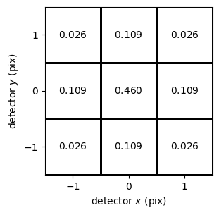
The charge diffusion kernel convolved with a pixel and then integrated over the extent of each pixel.

Parameters:

• width_diffusion (Quantity) – The standard deviation of the charge diffusion kernel. Often computed using charge_diffusion().

• width_pixel (Quantity) – The width of a pixel.

• axis_x (str) – The name of the horizontal axis.

• axis_y (str) – The name of the vertical axis.

Return type:

FunctionArray[Cartesian2dVectorArray, ScalarArray]

Examples

Plot this diffusion kernel

import matplotlib.pyplot as plt
import astropy.units as u
import named_arrays as na
import optika

# Define the wavelength to compute the charge diffusion kernel for.
wavelength = 1403 * u.AA

# Define the width of pixel
width_pixel = 13 * u.um

# Load the optical properties of silicon
si = optika.chemicals.Chemical("Si")

# Retrieve the absorption coefficient of silicon
# for the given wavelengths.
absorption = si.absorption(wavelength)

# Compute the standard deviation of the charge diffusion kernel
width_diffusion = optika.sensors.charge_diffusion(
    absorption=absorption,
    thickness_substrate=14 * u.um,
    thickness_depletion=8.7 * u.um,
)

# Compute the charge diffusion kernel.
kernel = optika.sensors.kernel_diffusion(
    width_diffusion=width_diffusion,
    width_pixel=width_pixel,
    axis_x="x",
    axis_y="y",
)

# Plot the charge diffusion kernel.
fig, ax = plt.subplots(
    figsize=(3, 3),
    constrained_layout=True,
)
na.plt.pcolormesh(
    kernel.inputs.x,
    kernel.inputs.y,
    C=kernel.outputs,
    facecolors="None",
    edgecolors="black",
)
na.plt.text(
    x=kernel.inputs.x,
    y=kernel.inputs.y,
    s=kernel.outputs.to_string_array(format_value="%.3f"),
    color="black",
    ha="center",
    va="center",
)
ax.set_xlabel("detector $x$ (pix)")
ax.set_ylabel("detector $y$ (pix)")
ax.set_aspect("equal")
ax.set_xticks([-1, 0, 1]);
ax.set_yticks([-1, 0, 1]);

References to optika.sensors.kernel_diffusion
kernel_diffusion