electrons_measured_approx

optika.sensors.electrons_measured_approx(photons_absorbed, wavelength, absorption=None, thickness_implant=<Quantity 2317. Angstrom>, thickness_substrate=<Quantity 7. um>, cce_backsurface=0.21, temperature=<Quantity 300. K>, iqy=None, fano_factor=None, shape_random=None)

A random sample from an approximate distribution of measured electrons given the number of photons absorbed by the light-sensitive layer of the sensor.

This function accounts for both Fano noise and recombination noise due to partial-charge collection.

Parameters:

• photons_absorbed (Quantity | AbstractScalar) – The number of photons absorbed by the light-sensitive layer of the sensor.

• wavelength (Quantity | ScalarArray) – The vacuum wavelength of the absorbed photons.

• absorption (None | Quantity | AbstractScalar) – The absorption coefficient of silicon per unit perpendicular depth. For oblique incidence, supply the effective coefficient from optika.sensors.absorption_effective(), which folds in the refracted angle, so no separate angle argument is needed.

• thickness_implant (Quantity | AbstractScalar) – The thickness of the implant layer, where partial-charge collection occurs.

• thickness_substrate (Quantity | AbstractScalar) – The thickness of the entire light-sensitive region of the device. The absorbed photons are distributed within this region, which sets the fraction that land in the implant layer.

• cce_backsurface (Quantity | AbstractScalar) – The differential charge collection efficiency on the back surface of the sensor.

• temperature (Quantity | ScalarArray) – The temperature of the silicon detector. Default is room temperature.

• iqy (None | Quantity | AbstractScalar) – The ideal quantum yield of the sensor in electrons per photon. If None (the default), the result of quantum_yield_ideal() is used.

• fano_factor (None | Quantity | AbstractScalar) – The Fano factor (ratio of the variance to the mean) of the Fano noise for this sensor material in units of electrons per photon. If None (the default), the result of fano_factor() is used.

• shape_random (None | dict[str, int]) – Additional shape used to specify the number of samples to draw.

Return type:

AbstractScalar

Examples

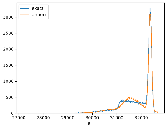
Plot the energy spectrum of twenty 6 keV photons emitted from an Fe-55 radioactive source and compare it to the exact spectrum

import matplotlib.pyplot as plt
import astropy.units as u
import astropy.visualization
import named_arrays as na
import optika

# Define the number of experiments to perform
num_experiments = 100000

# Define the expected number of photons
# for each experiment
photons_absorbed = (20 * u.photon).astype(int)

# Define the wavelength at which to sample the distribution
wavelength = 5.9 * u.keV
wavelength = wavelength.to(u.AA, equivalencies=u.spectral())

# Compute the actual number of electrons measured for each experiment
electrons_exact = optika.sensors.electrons_measured(
    photons_absorbed=photons_absorbed,
    wavelength=wavelength,
    shape_random=dict(experiment=num_experiments),
)

# Compute the approximate number of electrons measured for each experiment
electrons_approx = optika.sensors.electrons_measured_approx(
    photons_absorbed=photons_absorbed,
    wavelength=wavelength,
    shape_random=dict(experiment=num_experiments),
)

# Define the histogram bins
step = 10
bins = na.arange(
    electrons_exact.value.min()-step/2,
    electrons_exact.value.max()+step/2,
    step=step,
    axis="bin",
) * u.electron

# Compute a histogram of exact energy spectrum
hist_exact = na.histogram(
    electrons_exact,
    bins=bins,
    axis="experiment",
)

# Compute a histogram of approximate energy spectrum
hist_approx = na.histogram(
    electrons_approx,
    bins=bins,
    axis="experiment",
)

# Plot the histogram
with astropy.visualization.quantity_support():
    fig, ax = plt.subplots()
    na.plt.stairs(
        hist_exact.inputs,
        hist_exact.outputs,
        ax=ax,
        label="exact",
    );
    na.plt.stairs(
        hist_approx.inputs,
        hist_approx.outputs,
        ax=ax,
        label="approx",
    );
    ax.legend();

References to optika.sensors.electrons_measured_approx
electrons_measured_approx