absorbance

optika.sensors.absorbance(wavelength, direction=1, n=1, thickness_oxide=<Quantity 50. Angstrom>, thickness_substrate=<Quantity 7. um>, chemical_oxide='SiO2', chemical_substrate='Si', roughness_oxide=<Quantity 0. nm>, roughness_substrate=<Quantity 0. nm>, method='Beer-Lambert')

The fraction of incident energy absorbed by the light-sensitive region of the sensor

Parameters:

• wavelength (Quantity | AbstractScalar) – The wavelength of the incident light in vacuum.

• direction (float | AbstractScalar) – The cosine of the incidence angle. Default is normal incidence.

• n (complex | AbstractScalar) – The complex index of refraction in the ambient medium.

• thickness_oxide (Quantity | AbstractScalar) – The thickness of the oxide layer on the illuminated surface of the sensor. Default is the value given in Stern et al. [1994].

• thickness_substrate (Quantity | AbstractScalar) – The thickness of the light-sensitive substrate layer. Default is the value given in Stern et al. [1994].

• chemical_oxide (str | AbstractChemical) – The chemical formula of the oxide layer on the illuminated surface of the sensor. Default is silicon dioxide.

• chemical_substrate (str | AbstractChemical) – The chemical formula of the light-sensitive portion of the sensor. Default is silicon.

• roughness_oxide (Quantity | AbstractScalar) – The RMS roughness the oxide layer surface.

• roughness_substrate (Quantity | AbstractScalar) – The RMS roughness of the substrate surface.

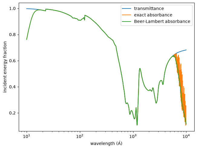
• method (Literal['exact', 'Beer-Lambert']) – The method to use to compute the absorbance. If exact, this method allows thin-film interference effects inside the light-sensitive region. If Beer-Lambert, this method assumes no interference effects. These methods only differ in the infrared, where the wavelength is commensurate with the thickness of the light-sensitive region.

Return type:

PolarizationVectorArray

Examples

Plot the absorbance as a function of wavelength and compare it to the transmittance.

import matplotlib.pyplot as plt
import astropy.units as u
import named_arrays as na
import optika

# Define a grid of wavelengths
wavelength = na.geomspace(10, 10000, axis="wavelength", num=1001) * u.AA

# Compute the transmittance vs wavelength
transmittance = optika.sensors.transmittance(
    wavelength=wavelength,
)

# Compute the absorbance vs wavelength
absorbance_exact = optika.sensors.absorbance(
    wavelength=wavelength,
    method="exact",
)

absorbance_beer = optika.sensors.absorbance(
    wavelength=wavelength,
    method="Beer-Lambert",
)

# Plot the average absorbance vs. wavelength
fig, ax = plt.subplots(constrained_layout=True)
na.plt.plot(
    wavelength,
    transmittance.average,
    ax=ax,
    label="transmittance",
);
na.plt.plot(
    wavelength,
    absorbance_exact.average,
    ax=ax,
    label="exact absorbance",
);
na.plt.plot(
    wavelength,
    absorbance_beer.average,
    ax=ax,
    label="Beer-Lambert absorbance",
);
ax.set_xscale("log");
ax.set_xlabel(f"wavelength ({wavelength.unit:latex_inline})");
ax.set_ylabel("incident energy fraction");
ax.legend();

References to optika.sensors.absorbance
absorbance